KNN and KD Trees

In machine learning, KNN (K-Nearest Neighbor, also known as the k-nearest neighbors algorithm) is a fairly simple model. It works by calculating the distance between data points and then classifying a set of data into k categories. It is a typical discriminative model.

My mentor used to say, this method is ridiculously simple. So why introduce it? Because when solving real-world problems, giving it a try and tuning its parameters often yields surprisingly good results—why not introduce it? Whether a method is simple or complex, the best one is the one with the highest F1-measure and the smallest computational cost. Some approaches involve all kinds of complex calculations and look incredibly profound, yet fail to explain anything convincing or prove themselves through F1-measure; those are only good for publishing papers.

Distance

First, let's define the concept of distance.

Suppose we have $x_i = (x_i^{(1)},x_i^{(2)},x_i^{(3)},...,x_i^{(n)})$ and $x_j = (x_j^{(1)},x_j^{(2)},x_j^{(3)},...,x_j^{(n)})$; how do we measure how different $x_i$ and $x_j$ are?

There is a definition $L_p$, namely the so-called $L_p$ distance or Minkowski distance. Its definition is as follows:

$L_p(x_i,x_j) = (\Sigma_{l=1}^{n}|x_i^{(l)} - x_j^{(l)}|^p)^{\frac{1}{p}}$

In other words, compute the absolute difference for each corresponding component, raise each to the p-th power, sum them all, and then take the $\frac{1}{p}$-th root.

For example, given dataset $x_1$=(1,2) and $x_2$=(3,4), assuming p is 3, now let's find the value of $L_3(x_1,x_2)$. The derivation is as follows:

$L_3(x_1,x_2) = (\Sigma_{l=1}^{n}|x_1^{(l)} - x_2^{(l)}|^3)^{\frac{1}{3}} \\\ = (|x_1^{(1)} - x_2^{(1)}| ^ 3 + |x_1^{(2)} - x_2^{(2)}| ^ 3 )^{\frac{1}{3}} \\\ = (|1-3| ^ 3 + | 2 - 4 | ^ 3) ^{\frac{1}{3}} \\\ = ( 2 ^ 3 + 2 ^ 3) ^{\frac{1}{3}} \\\ = (16) ^{\frac{1}{3}} \\\ = \sqrt[3]{16} \\\$

It's actually quite simple; if I weren't such a slow learner, the result would probably come straight out just by looking at this dataset.

• When p = 1, it has a special name, called Manhattan distance (Manhattan distance);
• When p = 2, it's called Euclidean distance (Euclidean distance);
• When p = 3, it's called Akekenwei distance (Joke distance);
• When p = $\infty$, it is the maximum of the coordinate distances, which is $L_\infty (x_i,x_j) = \max_i | x_i^{(l)} - x_j^{(l)}|$

Graphically, when p takes the values above, for a two-dimensional array, the boundary at distance "1" is roughly as shown below.

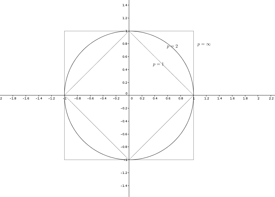
From a purely mathematical standpoint, we can generalize this formula to N-dimensional arrays of any finite length greater than 0. Thus, for any two N-dimensional arrays, we can always compute a value; the smaller this value, the closer the "distance" between the two points in N-dimensional space, meaning the higher the "similarity" between the two points.

From Points to Trees

However, up to now, the so-called distance has been between two points. Following this approach, if we have a dataset with 1000 records and we bring out the 1001st record, hoping to find the closest record among the previous 1000, we would seemingly need to compare 1000 times. This is obviously unacceptable. Clever predecessors came up with a special technique that lets us find the nearest data point with as few comparisons as possible. That is the KD-tree.

Using a KD-tree is actually quite simple.

First, we need to construct a KD-tree.

Taking a dataset {T1(2,3),T2(5,4),T3(9,6),T4(4,7),T5(8,1),T6(7,2)} as an example, the construction method is as follows:

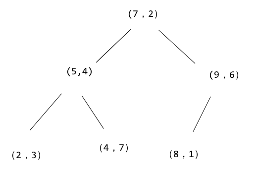
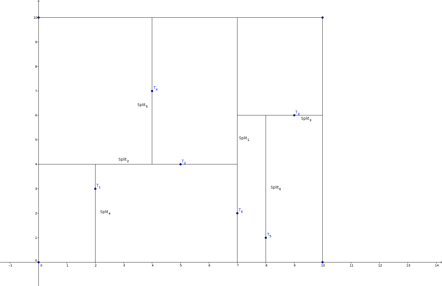
• S1: First, we sort the dataset by the first dimension of each data point and take the median. In this example, from {2,5,9,4,8,7}, we find the middle one, which is T6(7,2). To its left are {T1(2,3),T2(5,4),T4(4,7)}, and to its right are {T3(9,6),T5(8,1)}.
• S2: Then, for each split subset, we sort by the second dimension and take the median. For the left subset {3,4,7}, the root node is T2(5,4). For the right subset {6,1}, following the previous convention, if the subset has an even number of elements, we take the right one, so the root node is T3(9,6).
• S3: The third step should sort by the third dimension, but this dataset has only two dimensions, so we continue sorting by the first dimension.

Thus we finally obtain the following tree:

It can also be understood as follows:

Then, when a new data point arrives, we simply start from the root node and traverse down in the same way. If no exact match is found, we compare each node along the path with the new point. The complexity is $O(log_2n)$, which is much better than the previous $O(n)$.

Finally, I wrote a demo; you can click here to check it out. In short, it randomly generates some data points, builds a KD tree, then randomly creates a new data point and finds the closest one among the previous data.

Reference:

[1] Li Hang. Statistical Learning Methods[M]. Beijing: Tsinghua University Press, 2012.