Perceptron

The perceptron is a type of 机器学习(machine learning)–监督学习(supervised learning)–判别模型(discriminative model).

Supervised learning means that, given a training set $X_t$ and its corresponding result set $Y_t$, we train a model, and then when a new test set $X_p$ appears, we can obtain the predicted result $Y_p$.

A discriminative model is different from a Bayesian-based generative model (generative model); it assumes that you have a set of parameters $X = x_1,x_2,x_3...$, and the values of this set X are computed according to some formula to obtain the result $Y$.

Now suppose there is such a model where the relationship between X and Y is $Y = w_0 + w_1 * x_1 + w_2 * x_2 + w_3 * x_3 ...$; $X$ is a set of real numbers, so Y is naturally also a real-valued result.

But in practical use, suppose this is a binary classification problem; then set class a to -1 and class b to +1. The result obtained after training is unlikely to be exactly +1 or -1, so we map values greater than 0 to +1, i.e., b, and otherwise to a.

Thus, our problem is clear: based on the existing relationship from X to Y (that is, the training data), we need to train a set of W; substituting this set of W into the formula above yields a predicted Y.

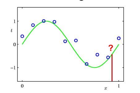
We get a distribution like the one above: the blue dots represent the scatter of x, and the green line shows the actual trend of y.

Now, we try to tune this set of parameters at each point so that the green line gets as close as possible to all the blue dots.

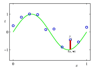
For a single point, we try to compute the distance between that point and the curve under the current W, as indicated by the red line.

We construct a loss function as follows:

$L(w) =\frac{1}{2} \sum_{i=1}^{N} {(f(x_i,w) - y_i)^2}$

The smaller the value of this loss function, the smaller the distance between the points and the line. So our goal is to find the W that minimizes L(w) according to this formula.

Gradient descent can come in handy here. For each element w of W, we can update it as follows:

$w_j = w_j - \Delta \frac{ \partial L(w)}{ \partial w_j}$

$\Delta$ represents the learning rate, $\frac{ \partial L(w)}{ \partial w_j}$

The partial derivative of L(w) with respect to the current w is the update ratio for the j-th element of W on the current dataset.

Then the process for computing $\frac{ \partial L(w)}{ \partial w_j}$ is as follows:

$\frac{ \partial L(w)}{ \partial w_j} = \frac{ \partial }{ \partial w_j} \frac{1}{2} (f(x,w)-y)^2 \\\ =(f(x,w) - y) \frac{ \partial }{ \partial w_j}( \sum_{j=0}^{M} x^j -y ) \\\ =(f(x,y) -y) x^j$

Therefore, $w_j = w_j - \Delta(f(x,y) -y)x^j$

That covers the rough theory. In practice, there are two kinds of gradient descent: BGD (batch gradient descent) and SGD (stochastic gradient descent). Since I’m in a hurry to grab dinner, I’ll fill in the details when I have time later.

Then I implemented it accordingly; there’s a simple implementation here. Feel free to take a look if you’re interested, although it’s pretty much useless in real-world applications.

All in all, this is a model with strong assumptions. If you’re sure that factors a, b, and c have a first-order effect on the result, using it is fine; but in reality, that’s only true in rare, ideal cases.

References

• Statistical Learning Methods, Hang Li, Beijing: Tsinghua University Press, 2012
• Advanced Machine Learning Lecture Notes, Jie Tang, Jun Zhu